
Exposure and Overhead
Time on Source
VLBA observers are responsible for creating their own schedules for each observation. There are two tools that can be used to determine what amount of time needs to be spent on the source(s) of interest for each observation: the new EVN Observation Planner or the old EVN Calculator.
Time on Source: EVN Observation Planner
The new EVN Observation Planner (also known as the "planobs tool") can be used in either a "Guided Mode" or a "Manual Mode". The Guided Mode makes some assumptions about your observation that may not be accurate, so NRAO recommends using the tool in Manual Mode.
To use the EVN Observation Planner in Manual Mode to estimate the time on source required to achieve your desired sensitivity, follow these steps:
- Select the antennas to use. It is usually easiest to use the “Select default VLBA Network(s)” drop-down menu to select all of the VLBA antennas first. You can add or remove antennas at any time. Remember to only select the minimum number of antennas you specified are necessary for your project.
- Select the observing band.
- Select from the options under “Source and Epoch”. If the source and epoch are both known, select "Define source and epoch" and enter the source and epoch information. If either the source or the epoch is unknown, select "Do not specify source or epoch".
- Enter the duration of the observation in hours.
- Under “% of on-target time”, move the marker to your estimate of the percent of the total observation duration that the target will be observed (default is 70%, which may be a bit optimistic).
- Select the desired data rate. For most continuum observations at 5 GHz or higher, this should be "4 Gbps". If you are observing at L (21 cm, 1 GHz) or S (13 cm, 2 GHz) bands, you should select "2 Gbps".
- Select the number of subbands. For the VLBA, the DDC personality allows up to 8 subbands total. If you are using dual or full polarization, that means 4 subbands per polarization. The PFB personality uses 32 subbands (16 per polarization in dual and full polarization).
- Select the number of spectral channels. This will not impact the sensitivity, but it will impact the available field of view and the output file size. If the field of view is too small due to bandwidth smearing, increase the number of spectral channels. For 4 Gbps mode, the NRAO recommends 256 or 512 spectral channels. (Check the “FoV limitations” section of the output summary to make sure that the FoV limits for time and frequency smearing are comparable.)
- Select the number of polarizations.
- Select the integration time (the default is 2 seconds, which is the default VLBA integration time a well).
- Click “COMPUTE” in the upper-left of the page. The tool will make the calculations based on your inputs and display a summary of the results. You can change any of the inputs and re-compute at any time.
Once the tool has finished computing the observation, check the "Sensitivity" box on the Summary tab. If the calculated sensitivity is not what you need, change the duration of the observation and compute again. Adjust until the sensitivity matches your needs.
If you entered the coordinates for you target, you should also check the "Elevations" tab to see estimates of when the object will be visible from the selected antennas.
Once you are satisfied with the sensitivity estimate, click on the "DOWNLOAD SUMMARY AS PDF" link on the Summary tab (near the top of the page, just under the tabs). This will provide you with a document you can include in your Technical Justification.
Time on Source: Old EVN Calculator
To use the old EVN Calculator to estimate the time on source required to successfully complete a project, follow these steps.
- Station Selection (upper left)
Click on the “VLBA” button in the top left section of the calculator. This will automatically select all of the VLBA stations. It is usually a good idea to de-select one or two stations, under the assumption that something will happen to at least one antenna during a real observation (maintenance work, poor weather, mechanical or computer issues, etc.). Most observers assume that they will have 8 antennas available at any given time. If you are proposing for a VLBA-plus project (HSA, GMVA, or global VLBI), make sure to select the extra stations. Remember to only select the minimum number of antennas you specified are necessary for your project. - Observing band & data rate selection (upper left)
Select the observing band you want to use for your observation. If you will be observing with multiple bands, you will need to do the calculation for each band separately.
Select the data rate you wish to use. For most VLBA continuum observations, the default data rate is now 2048 Mbps. If you want the best possible continuum sensitivity at wavelengths of 6cm or shorter, select 4096 Mbps. - Select the number of spectral channels per subband, integration time, and maximum baseline length (lower left)
These settings will not affect the sensitivity, but they will affect the field of view and the FITS file size. If you plan to use the polyphase filterbank (PFB) observing system, the default is 64 channels. If you plan to use the digital down conversion (DDC) observing system, the default is 256 channels. You are free to choose however many spectral channels you prefer. The default integration time for the VLBA is 2 seconds. For standard VLBA observing, the maximum baseline should be set to 9000 km. - Select the number of polarizations, subbands per polarizations, and bandwidth (lower right). The default number of polarizations for the VLBA is 2, but 1 or 4 can also be used.
If you will be using the polyphase filter bank (PFB) observing system, the number of polarizations times the number of subbands per polarization must be 16 and the bandwidth must be 32 MHz.
If you will use the digital down conversion (DDC) system, you can choose nearly any setup you prefer as long as the number of subbands per polarization is 8 or fewer.
Note: The calculator tool will warn you if your selected number of polarizations, subbands, and bandwidth do not match your selected data rate (from step 2). - Enter an on-source integration time in minutes (upper right) then click “GO” (upper right or lower right). The tool will estimate the image thermal noise you can expect for your setup and on-source integration time. Note that this does not take into account the effects of side lobes, scattering, or radio frequency interference (RFI). Also, keep in mind that observations at low elevations may have higher than usual noise.
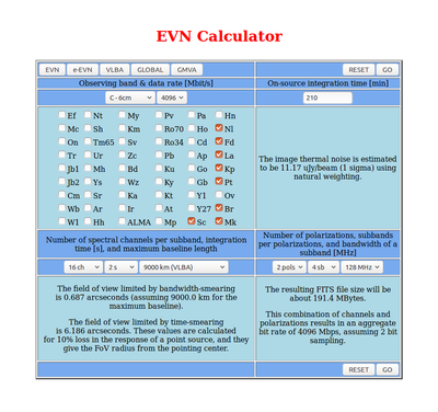
Save screen shots of your EVN Calculator results (see the example below) to attach to your proposal in the Technical Justification section.
 |
|---|
| Example of using the EVN Exposure Calculator. Notice that only 8 antennas are selected. This is because the (hypothetical) proposal states that a minimum of 8 antennas are required for the project to be successful. |
Time on Source: Note for 3mm Observations
The 3mm noise estimates provided by both the EVN Observation Planner and the old EVN Calculator use System Equivalent Flux Density (SEFD) values determined during reasonably good weather and while the antennas were performing well. Because real-world conditions are often less than ideal, the actual noise levels obtained during 3mm observations may be significantly worse. This is especially true for GMVA observations, which are observed on fixed dates and cannot be rescheduled due to poor weather. When planning for GMVA observations, users are encouraged to assume the actual noise values will be roughly 3 times higher than the tool's estimate.
Time on Source: Subbands vs Basebands
There is a subtle difference between how the sensitivity calculator tools and the NRAO PST Resources determine data rates. Both the EVN Observation Planner and the old EVN Calculator ask you to input the number of polarizations and subbands, while the PST Resources ask for the number of polarizations and data channels (formerly called "baseband channels"). Keep in mind that the number of data channels = (number of observed polarizations) x (number of subbands). In other words, for dual polarization, each subband has one left-hand circularly polarized (LCP) data channel and one right-hand circularly polarized (RCP) data channel. For full polarization (“4 pols”), only 2 polarizations are recorded during the observation and the cross-hand polarizations are determined during correlation, so the recorded data rates for “2 pols” and “4 pols” are identical.
To use either the EVN Observation Planner or the EVN Calculator to simulate a 4 Gbps DDC dual-polarization observation: select 4 subbands, 256 (or more) spectral channels per subband, and 2 polarizations.
To simulate a dual-polarization PFB observation: select 16 subbands, 64 (or more) spectral channels per subband, and 2 polarizations.
Time on Source: Spectral Line Observations
The EVN Calculator was designed primarily for continuum observations. If your project involves spectral line observations, you will need to make some additional calculations to estimate the noise in each spectral channel. The per-spectral-channel noise is the noise for the full bandwidth multiplied by the square root of the total number of spectral channels.
For example, assume you observe with 8 data channels per polarization and a data channel bandwidth of 32 MHz. If you want 125 kHz spectral channels, you will need to have 2048 spectral channels in each data channel (8 x 32 MHz / 125 kHz = 256 MHz/125 kHz = 2048). So, the per-spectral-channel noise would be the noise for the full bandwidth times the square root of 2048.
The new EVN Observation Planner provides the per-spectral-channel sensitivity along with the continuum sensitivity.
Time on Source: U-V Coverage
For some projects, particularly those attempting to image complicated structures, filling in as much of the u-v plane as possible may be a greater concern than the sensitivity. If this is the case for your project, be sure to make a note of this in the Technical Justification. Note that the EVN Observation Planner provides an estimate of the u-v coverage for an observation on the UV Coverage tab.
Full Bandwidth vs. Usable Bandwidth
Continuum observations at lower frequencies (at wavelengths of about 13 cm and longer) often encounter problems with RFI. In some cases, large portions of the bandwidth are completely dominated by RFI and are unusable for science. If you are proposing for a low frequency project, it is prudent to assume that the usable bandwidth will be substantially reduced (by up to about 30%). Therefore, the time on source necessary to achieve your desired image thermal noise will be significantly longer than the EVN Observation Planner predicts. If you are asking for more time than the EVN Observation Planner predicts is necessary, make sure to explain why in the Technical Justification.
For example, "The EVN Observation Planner predicts a time on source of 120 minutes will result in an image thermal noise of 25 microJy/beam. However, this is assuming the entire 256 MHz, dual polarization bandwidth at 21 cm will be usable. We anticipate that approximately 30% of the bandwidth will be unusable due to RFI, and therefore we will require 172 minutes on source to reach the necessary signal-to-noise ratio."
Overhead and Total Time
When proposing for time on the VLBA (and other NRAO telescopes), you must request the total time needed for the entire project. This is not just the time on science targets. It also includes time for observing calibrators, time slewing between sources, and the time it takes to change from one frequency setup to another (if you are observing with multiple bands in a single observation).
Estimating Total Observing Time
A “rule of thumb” is that, for a phase referencing observation, the time spent on the science target will be roughly 60% to 70% of the total observing time. The other 30% to 40% of the time will be spent slewing and observing calibration sources. So, to make a conservative estimate of the total observing time you would divide the desired on-source time by 0.6. However, users should be extremely cautious about blindly using this estimate. It only works for projects at low frequencies observing a single science target and phase reference calibrator. Most observers also schedule time on a "check source", a known bright source that can be used to test how well the calibration worked. If your project involves multiple science targets, the project will have more slew time. If your project requires polarimetry, you will also need to schedule scans on polarization leakage (D-term) and electric vector polarization angle (EVPA) calibrator targets. If your phase reference calibrator is relatively far from your science target, the slew time will be longer. If you are observing at high frequencies, you will need to cycle back and forth between the phase reference calibrator and the science target at a higher cadence which adds more slew time. In other words, the more complicated a project, the more overhead it will require.
The best way to estimate the total observing time is to build a dummy schedule with SCHED (see Chapter 6). If you do not know the location of your science target (e.g., for a triggered target of opportunity project), make some reasonable assumptions about where it could be (e.g., classical novae are most likely to be located near the Galactic Center). Then, make some assumptions that would add complications to the schedule. For example, assume that the science target does not have a phase reference calibrator very near by so the slew times will be longer.
To get started, you may use this example dummy.key scheduling file for a hypothetical phase referenced project. In the "In line source catalog", change the DUMMYTARGET source to your science target (and add others as needed). In "The Scans" section at the end, check that that all of your sources are included in the first group and make sure to change the group number if you have more than one science target. Change the phase reference source and check source to something realistic for your project. You will probably need to change the start time and/or date in the "Initial Scan Information" section, as well.
Note that the dummy.key file is built for a “typical” 5 GHz phase referenced observation with 3-minute scans on the science target and 2-minute scans on the phase reference calibrator. This assumes that the phase reference calibrator is relatively dim and requires 2 minute scans to achieve the necessary signal-to-noise ratio of 7. Many observers use significantly shorter scans on the phase reference calibrator, with scans as short as 30 seconds reasonable for brighter calibrator sources.
The cycle time (a.k.a. “switching time”) for a phase referenced observation is the time between the midpoints of two successive scans on the phase reference calibrator with one scan on the science target in between (i.e., cal, sci, cal). The cycle time should be no longer than the coherence time, which depends on your observing frequency. The dummy.key file assumes a coherence time of about 5 minutes: (120 seconds on phase calibrator)/2 + 180 seconds on science target + (120 seconds on phase calibrator)/2 = 300 seconds = 5 minutes. For frequencies below 1 GHz, assume a coherence time of about 2 minutes. At frequencies between 1 and 3 GHz, assume the coherence time is about 5 minutes. For frequencies at or above 5 GHz, you can estimate the coherence time using t[seconds] ~ 2600/frequency[GHz] (e.g., Moran & Dhawan 1995). Observers who want a more conservative estimate of the coherence time should consult Reid & Honma (2014). Also, keep in mind that the coherence time depends on the elevation of the source, with observations at lower elevations having shorter coherence times (e.g., Ulvestad 1999).
Once you have made all the changes to the dummy schedule, run SCHED on it by typing
sched < dummy.key
and inspect the summary (dummy.sum) file to see the total time for the observation (“Elapsed time for project”) and the total time on your science target(s). Change the number of repetitions (rep=#) and/or dwell times under "The Scans" and re-run SCHED until you settle on a schedule that gives you the desired time on your science target(s).
If you have any questions about determining the on-source time, building a dummy schedule, or running SCHED, please contact the VLBA staff via the helpdesk.

